Cancer Transcriptome Example

Diagnostic Transcriptome Example

Used in Bio153H lecture using data from https://www.nature.com/articles/sdata2018136 A merged lung cancer transcriptome dataset for clinical predictive modeling. Original data was differential expression values of ~10,000 genes of ~1,000 patients with each patient being categorized as lung cancer positive or negative.

Data was preprocessed using the boruta package in r and the top 10 most important genes were selected from the total ~10,000 genes. Data was split into a training set and validation set. Various algorithms were trained and the best was tested against the confusion matrix of the validation set.

1 means cancer positive 2 means cancer negative

library(caret)

## Loading required package: lattice

## Loading required package: ggplot2

library(lattice)
library(e1071)
library(kernlab)

## 
## Attaching package: 'kernlab'

## The following object is masked from 'package:ggplot2':
## 
##     alpha

dataset1 <- read.csv("C:\\data\\CancerTranscriptomeTransposedImportance.csv", header = T, sep=",", colClasses = c('numeric'))
dataset1$Disease<-as.factor(dataset1$Disease)
validation_index <- createDataPartition(dataset1$Disease, p=0.80, list=FALSE)

validation <- dataset1[-validation_index,]
dataset1 <- dataset1[validation_index,]


# Run algorithms using 10-fold cross validation
control <- trainControl(method="cv", number=10)
metric <- "Accuracy"


set.seed(7)
fit.lda <- train(Disease~., data=dataset1, method="lda", metric=metric, trControl=control)

# b) nonlinear algorithms
# CART
set.seed(7) 
fit.cart <- train(Disease~., data=dataset1, method="rpart", metric=metric, trControl=control) 

# kNN
set.seed(7)
fit.knn <- train(Disease~., data=dataset1, method="knn", metric=metric, trControl=control)

# c) advanced algorithms
# SVM
set.seed(7)
fit.svm <- train(Disease~., data=dataset1, method="svmRadial", metric=metric, trControl=control) 
# Random Forest
set.seed(7)
fit.rf <- train(Disease~., data=dataset1, method="rf", metric=metric, trControl=control) 


# summarize accuracy of models
results <- resamples(list(lda=fit.lda, cart=fit.cart, knn=fit.knn, svm=fit.svm, rf=fit.rf))


# compare accuracy of models
dotplot(results)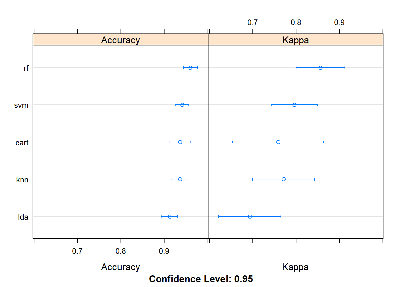

# estimate skill of LDA on the validation dataset
predictions <- predict(fit.rf, validation)
confusionMatrix(predictions, validation$Disease)

## Confusion Matrix and Statistics
## 
##           Reference
## Prediction   1   2
##          1 184   4
##          2   0  34
##                                           
##                Accuracy : 0.982           
##                  95% CI : (0.9545, 0.9951)
##     No Information Rate : 0.8288          
##     P-Value [Acc > NIR] : 1.555e-13       
##                                           
##                   Kappa : 0.9337          
##                                           
##  Mcnemar's Test P-Value : 0.1336          
##                                           
##             Sensitivity : 1.0000          
##             Specificity : 0.8947          
##          Pos Pred Value : 0.9787          
##          Neg Pred Value : 1.0000          
##              Prevalence : 0.8288          
##          Detection Rate : 0.8288          
##    Detection Prevalence : 0.8468          
##       Balanced Accuracy : 0.9474          
##                                           
##        'Positive' Class : 1               
##